Audio signals

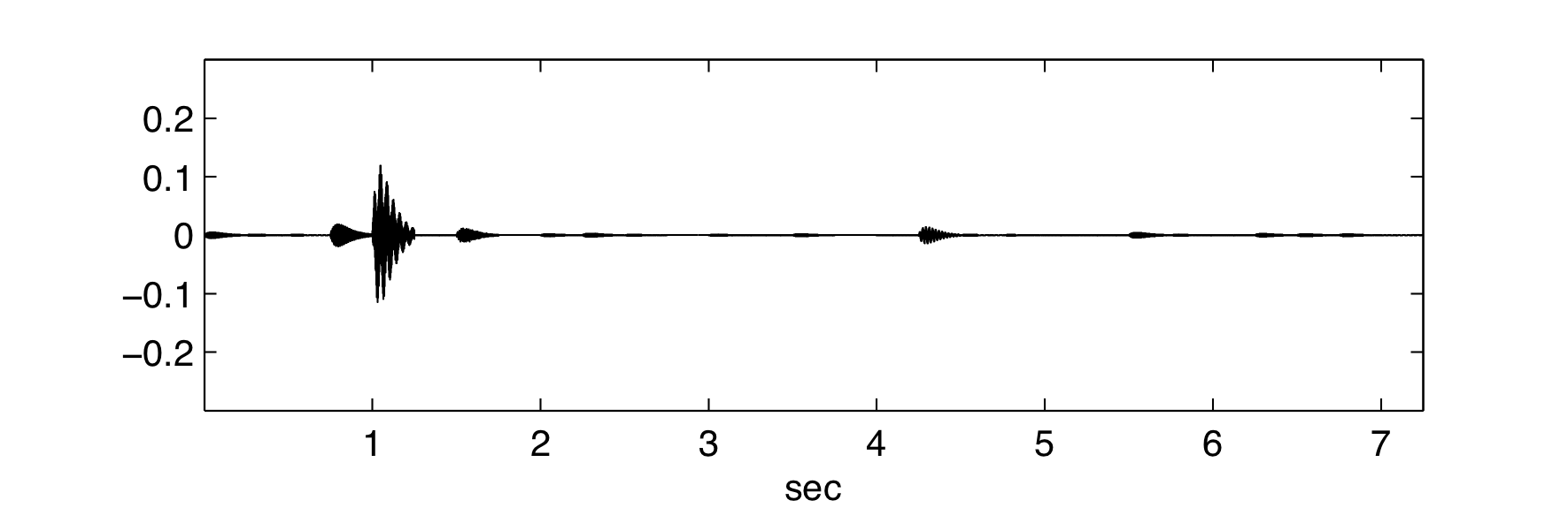
When represented in terms of appropriate elements, most signals have relatively few nonzero coefficients and hence are compressible. We illustrate the new procedure to reconstruct a signal from only a fraction of the number of samples required traditionally, on a simple audio file taken from here and we compare the results with the ones obtained using compressed sensing. A song containing 29 notes, each lasting 0.25 seconds and each decaying according to the same model, is sampled industrially at M = 44100 Hz. The result is a data vector of 319725 entries or 11025 samples per note. The 100 valid frequencies, which form a pianobasis, vary between 16.35 and 4978.03. Let us first illustrate the workings of compressed sensing to conclude with our new result.

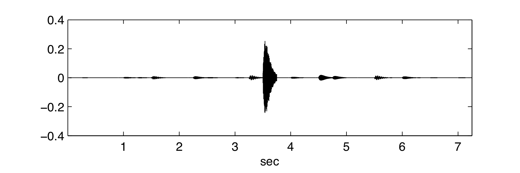
When undersampling the song randomly at about 42 samples per note (1229 samples in total), a reconstruction following the compressed sensing principle reveals a combination of piano basis frequencies that approximates the song quite well.

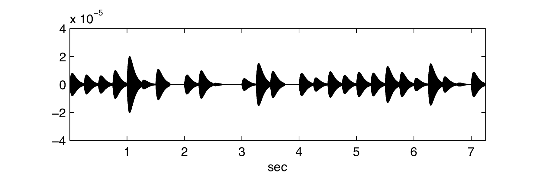
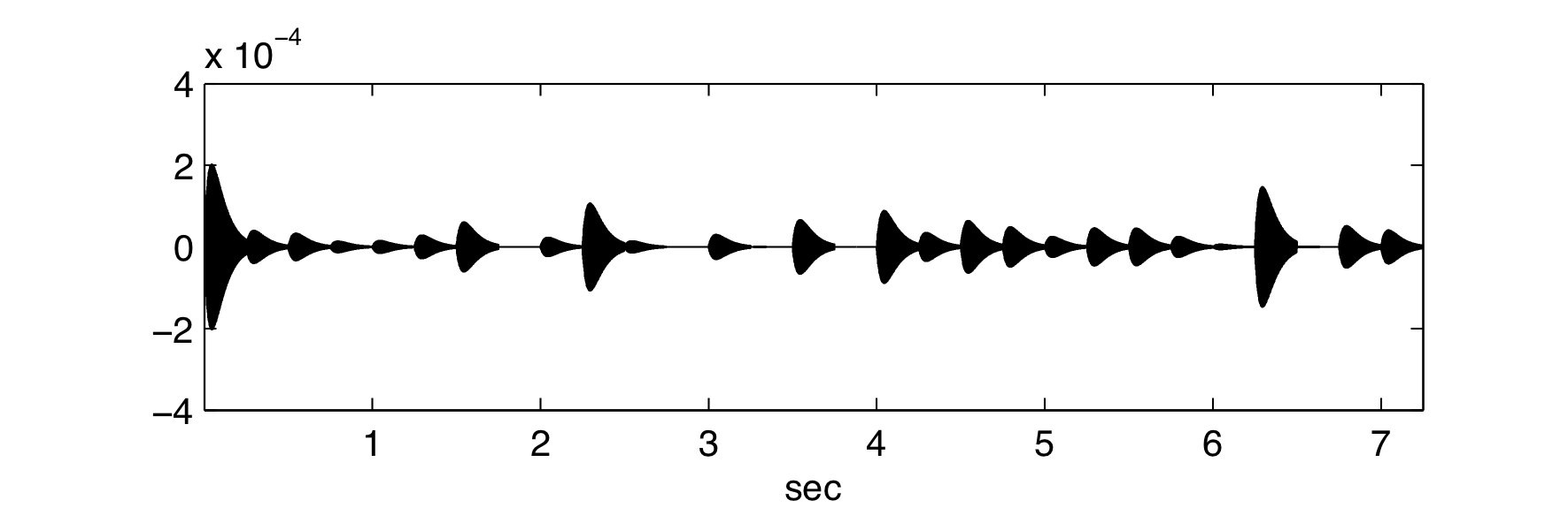
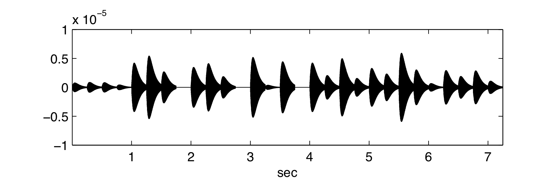
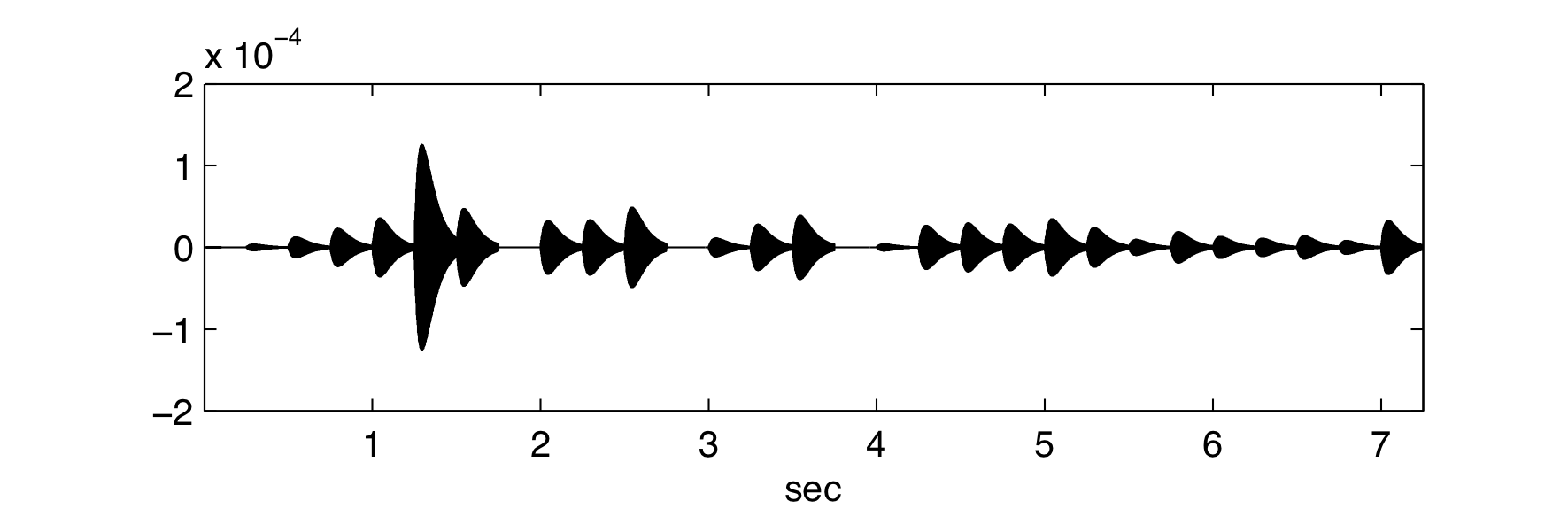
Because of the randomness in the sampling, the reconstructed signal may vary. To illustrate the probabilistic aspect of the compressed sensing technique, we plot the resulting error curves for the reconstructed signal compared to the original song, obtained in 4 different runs. The error curves confirm that the reconstruction is almost perfect: errors are of the magnitude of 10⁻⁴ to 10⁻⁵ on average.

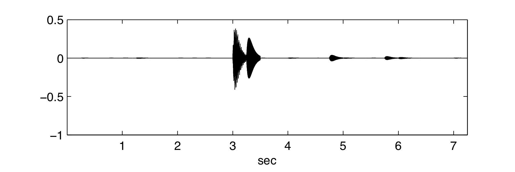
When repeating the experiment with only about 16 random samples per note (456 samples in total), the reconstruction using the compressed sensing technique fails, as can be seen from the error curves which are now of the magnitude of 10⁻¹.

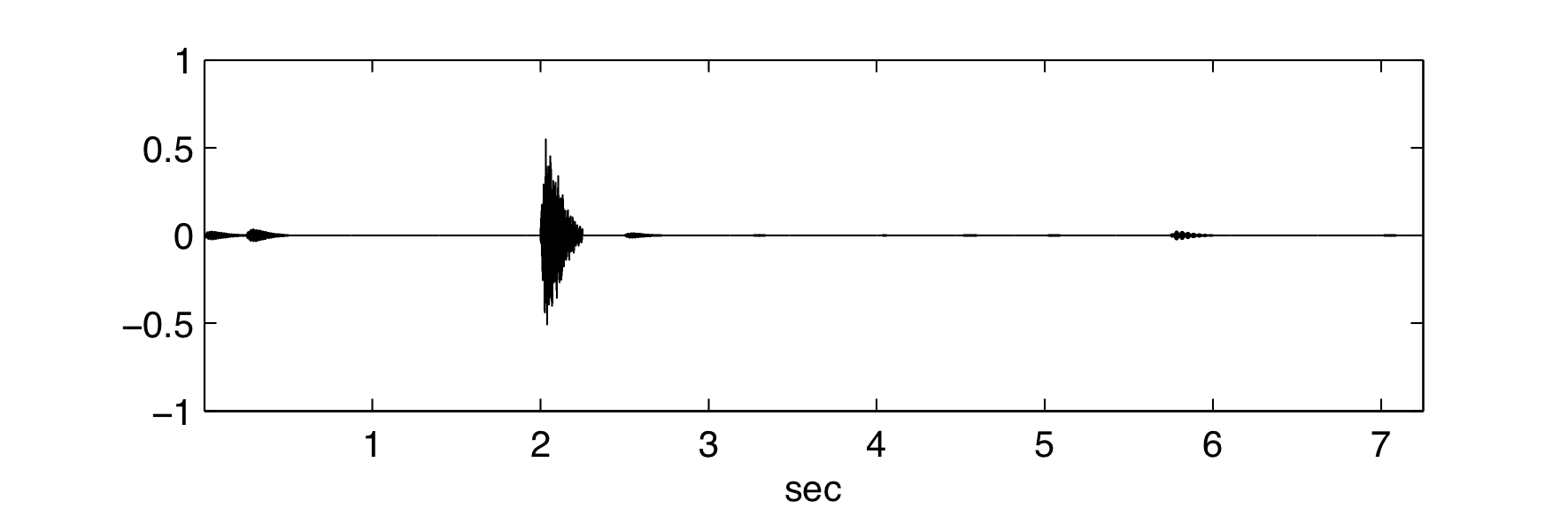
With the new technique, all frequencies can be retrieved exactly and the error curve is of the order of machine precision. But what is most remarkable is that per note only 5 samples are necessary, resulting in a total of only 145 samples for a perfect reconstruction (the error is of the order of machine precision)!